4. Data exploration and visualisation
Juergen Niedballa (camtrapr@gmail.com)
2024-02-01
Source:vignettes/camtrapr4.Rmd
camtrapr4.RmdOverview
camtrapR can help with data exploration by creating maps of observed species richness and the number of independent detections by species. It can also plot single-species and two-species diel activity data. In addition, a survey report summarising camera trap station operation and species records can be created easily. The usage of these functions will be demonstrated using the sample data set included in the package.
In creating the plots and the report, the species record table and the camera trap station information table are combined. Therefore, both are required as function input (more details in the vignette on “Image organisation and species/individual identification”).
Species presence maps
The function detectionMaps can generate maps of observed
species richness (number of different species recorded at stations) and
maps showing the number of observations by species. It uses the record
table produced by recordTable and the camera trap station
table as input. Note that the examples are not particularly pretty
because of the low number of records used in the sample data set.
Number of observed species
We first create a map of the number of observed species.
Mapstest1 <- detectionMaps(CTtable     = camtraps,
                          recordTable  = recordTableSample,
                          Xcol         = "utm_x",
                          Ycol         = "utm_y",
                          stationCol   = "Station",
                          speciesCol   = "Species",
                          printLabels  = TRUE,
                          richnessPlot = TRUE,    # by setting this argument TRUE
                          speciesPlots = FALSE,
                          addLegend    = TRUE
)
Number of records by species
Maps of the number of independent detections of the observed species
can be generated just as easily. Normally, maps for all species will be
created at once. Here, to avoid cluttering the vignette, we look at one
species only. This is achieved via the argument
speciesToShow. Arguments richnessPlot and
speciesPlots are changed compared to the observed species
richness plot above. It is also possible to set both arguments to TRUE
or FALSE.
 # subset to 1 species
recordTableSample_PBE <- recordTableSample[recordTableSample$Species == "PBE",]

 Mapstest2 <- detectionMaps(CTtable      = camtraps,
                           recordTable   = recordTableSample_PBE,
                           Xcol          = "utm_x",
                           Ycol          = "utm_y",
                           stationCol    = "Station",
                           speciesCol    = "Species",
                           speciesToShow = "PBE",     # added
                           printLabels   = TRUE,
                           richnessPlot  = FALSE,     # changed
                           speciesPlots  = TRUE,      # changed
                           addLegend     = TRUE
)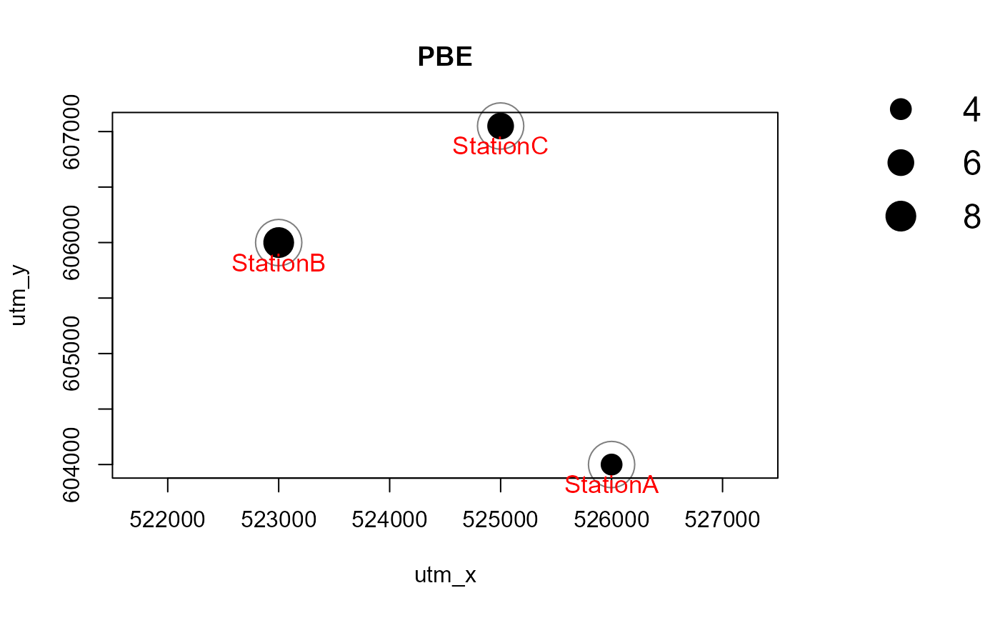
The number of independent observations depends on the argument
minDeltaTime in the recordTable function.
Shapefile export
Function detectionMaps comes with 4 arguments that allow
for and control creation of ESRI shapefile for use in GIS software:
writeShapefile, shapefileName,
shapefileDirectory and shapefileProjection.
The resulting shapefile will show stations as point features (as the map
above), with coordinates, total species number and number of
observations per species in the attribute table. The shapefile attribute
table is identical to the resulting data.frame of the
detectionMaps function.
The following example demonstrates the creation of a shapefile using
detectionMaps. Please note that for demonstration the
shapefile is saved to a temporary directory, which makes no sense in
real data and must be changed by the user. The argument
shapefileProjection must be a valid argument to the
function st_crs from the package sf. It can be
one of one of (i) character: a string accepted by GDAL, (ii) integer, a
valid EPSG value (numeric), or (iii) an object of class crs.
In contrast to previous versions, the EPSG code is the easiest way to pass the coordinate system information. These can be found under https://spatialreference.org/. In this case, it’s UTM zone 50N in WGS84 ellipsoid. In this case the EPSG code is 32648. You can provide the projection information as one of (i) character: a string accepted by GDAL, (ii) integer, a valid EPSG value (numeric), or (iii) an object of class crs.
Because it is so widespread, here’s the PROJ4 string for standard Lat/Long coordinates using the WGS84 ellipsoid (a standard used by most GPS devices): EPSG:4326, or "+proj=longlat +ellps=WGS84 +datum=WGS84 +no_defs".
 # define shapefile name
 shapefileName       <- "recordShapefileTest"

# projection: WGS 84 / UTM zone 50N = EPSG:32650
# see: https://spatialreference.org/ref/epsg/32650/
 shapefileProjection <- 32650

# run detectionMaps with shapefile creation
Mapstest3 <- detectionMaps(CTtable            = camtraps,
                          recordTable         = recordTableSample,
                          Xcol                = "utm_x",
                          Ycol                = "utm_y",
                          stationCol          = "Station",
                          speciesCol          = "Species",
                          richnessPlot        = FALSE,         # no richness plot
                          speciesPlots        = FALSE,         # no species plots
                          writeShapefile      = TRUE,          # but shaepfile creation
                          shapefileName       = shapefileName,
                          shapefileDirectory  = tempdir(),     # change this in your scripts!
                          shapefileProjection = shapefileProjection
)
## Writing layer `recordShapefileTest' to data source
## `C:\Users\niedballa\AppData\Local\Temp\Rtmp4eq9ph' using driver `ESRI Shapefile'
## Writing 3 features with 7 fields and geometry type Point.
# check for the files that were created
list.files(tempdir(), pattern = shapefileName)
## [1] "recordShapefileTest.dbf" "recordShapefileTest.prj"
## [3] "recordShapefileTest.shp" "recordShapefileTest.shx"
# if writeShapefile = TRUE the output is a sf object
Mapstest3
## Simple feature collection with 3 features and 7 fields
## Geometry type: POINT
## Dimension: XY
## Bounding box: xmin: 523000 ymin: 604000 xmax: 526000 ymax: 607050
## Projected CRS: WGS 84 / UTM zone 50N
## Station EGY MNE PBE TRA VTA n_species geometry
## 1 StationA 0 0 4 0 2 2 POINT (526000 604000)
## 2 StationB 0 2 8 0 2 3 POINT (523000 606000)
## 3 StationC 6 0 6 8 1 4 POINT (525000 607050)## Reading layer `recordShapefileTest' from data source
## `C:\Users\niedballa\AppData\Local\Temp\Rtmp4eq9ph' using driver `ESRI Shapefile'
## Simple feature collection with 3 features and 7 fields
## Geometry type: POINT
## Dimension: XY
## Bounding box: xmin: 523000 ymin: 604000 xmax: 526000 ymax: 607050
## Projected CRS: WGS 84 / UTM zone 50N
# we have a look at the attribute table
detections_sf
## Simple feature collection with 3 features and 7 fields
## Geometry type: POINT
## Dimension: XY
## Bounding box: xmin: 523000 ymin: 604000 xmax: 526000 ymax: 607050
## Projected CRS: WGS 84 / UTM zone 50N
## Station EGY MNE PBE TRA VTA n_species geometry
## 1 StationA 0 0 4 0 2 2 POINT (526000 604000)
## 2 StationB 0 2 8 0 2 3 POINT (523000 606000)
## 3 StationC 6 0 6 8 1 4 POINT (525000 607050)
# the output of detectionMaps is used as shapefile attribute table. Therefore, they are identical:
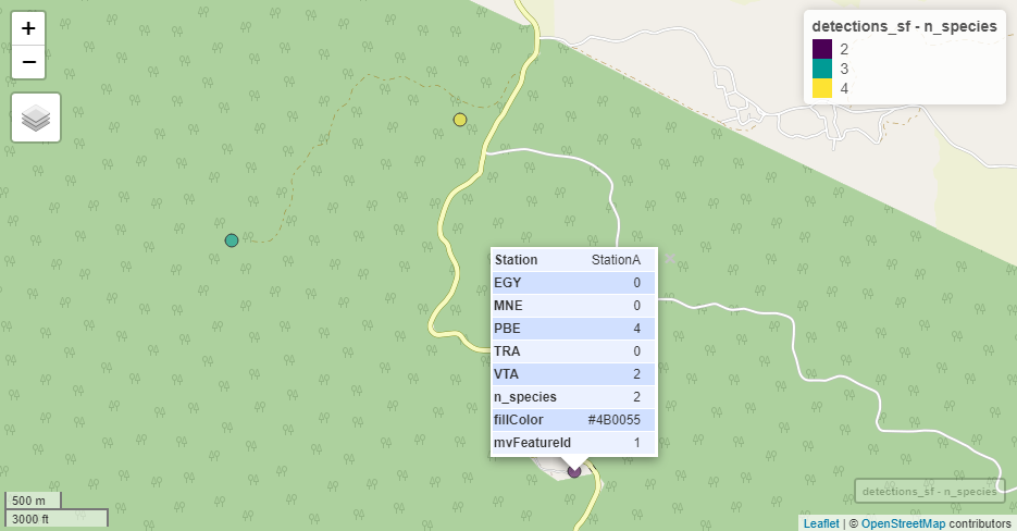
all(detections_sf == Mapstest3)## [1] TRUEA simple way of plotting these data in a map is via the mapview package. It opens an interactive map window, so it is not shown in this vignette.
One can also modify color or size of the points by values, e.g.
mapview(detections_sf,
        zcol = "n_species",
        cex  = "n_species")
The map viewer is interactive and allows different base maps, including satellite imagery. Here is an example with OpenStreetMap:
Using the output of detectionMaps for extracting covariate values from rasters
If writeShapefile = TRUE, the output of detectionMaps is a sf object (a data frame with a geometry column contain the spatial information). It can be used for extracting values from rasters for use as covariates.
# create a sample raster and extract data from it (if the raster package is available)
if("terra" %in% installed.packages()){
  library(terra)
  raster_test <- rast(extend(ext(detections_sf), y = 500),
                      nrows = 10, ncols = 10)
  values(raster_test) <- rpois(n = 100, lambda = seq(1, 100))    # fill raster with random numbers

  # plot raster
  plot(raster_test,
       main = "some raster with camera trap stations",
       ylab = "UTM N",     # needs to be adjusted if data are not in UTM coordinate system
       xlab = "UTM E")     # needs to be adjusted if data are not in UTM coordinate system

  # add points to plot
  points(detections_sf, pch = 16)

  # add point labels
  text(x      = st_coordinates(detections_sf)[,1],
       y      = st_coordinates(detections_sf)[,2],
       labels = detections_sf$Station,
       pos = 1)

  # extracting raster values. See ?extract for more information
  detections_sf$raster_value <- extract(x = raster_test, y = detections_sf)

  # checking the attribute table
  detections_sf

}
## terra 1.7.55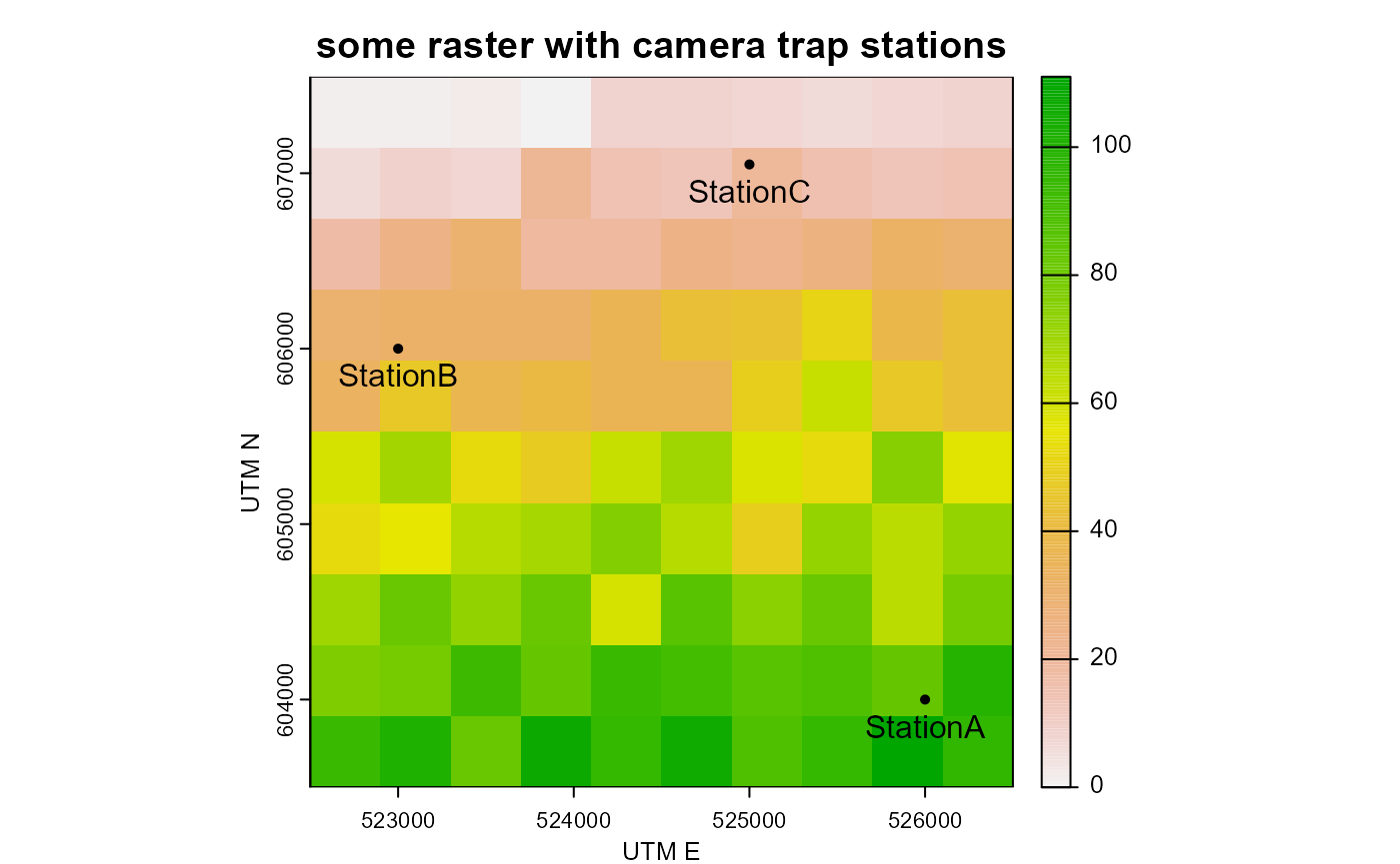
## Simple feature collection with 3 features and 8 fields
## Geometry type: POINT
## Dimension:     XY
## Bounding box:  xmin: 523000 ymin: 604000 xmax: 526000 ymax: 607050
## Projected CRS: WGS 84 / UTM zone 50N
##    Station EGY MNE PBE TRA VTA n_species              geometry raster_value.ID
## 1 StationA   0   0   4   0   2         2 POINT (526000 604000)               1
## 2 StationB   0   2   8   0   2         3 POINT (523000 606000)               2
## 3 StationC   6   0   6   8   1         4 POINT (525000 607050)               3
##   raster_value.lyr.1
## 1                 83
## 2                 31
## 3                 20
The same procedure also works with the camera trap station
information table instead of the detectionMaps output.
Visualising species activity data
Four different functions are provided to plot single-species and
two-species activity patterns. Activity data are visualised using the
time of day records were taken while ignoring the date. Record times are
read from the record table created by recordTable. The
criterion for temporal independence between records in the function
recordTable, minDeltaTime, will affect the
results of the activity plots. Imagine you make recordTable
return all records by setting minDeltaTime = 0 and you then
plot activity of some species that loves to perform in front of cameras
(e.g. Great Argus pheasants in Borneo), resulting in hundreds of images.
The representation of activity will be biased towards the times the
species happened to perform in front of your cameras. Likewise, setting
cameras to shoot sequences of several images per trigger event and then
returning all images will cause biased representations. Therefore, it is
wise to set minDeltaTime to some higher number, e.g. 60
(minutes).
If desired, all functions can save the plots as png files by setting
argument writePNG = TRUE.
Single-species activity plots
Single-species activity can be plotted in 3 different ways using 3 different functions:
-
activityDensity: kernel density estimation -
activityHistogram: histogram of hourly activity -
activityRadial: radial plot of hourly activity
In all three, users can either plot activity of one focal species (by
setting argument allSpecies = FALSE) or of all recorded
species at once (by setting argument allSpecies = TRUE). If
desired, plots can be saved as png files in a user-defined location
automatically (arguments writePNG and
plotDirectory). Note that the examples are not particularly
pretty because of the low number of records used in the sample data
set.
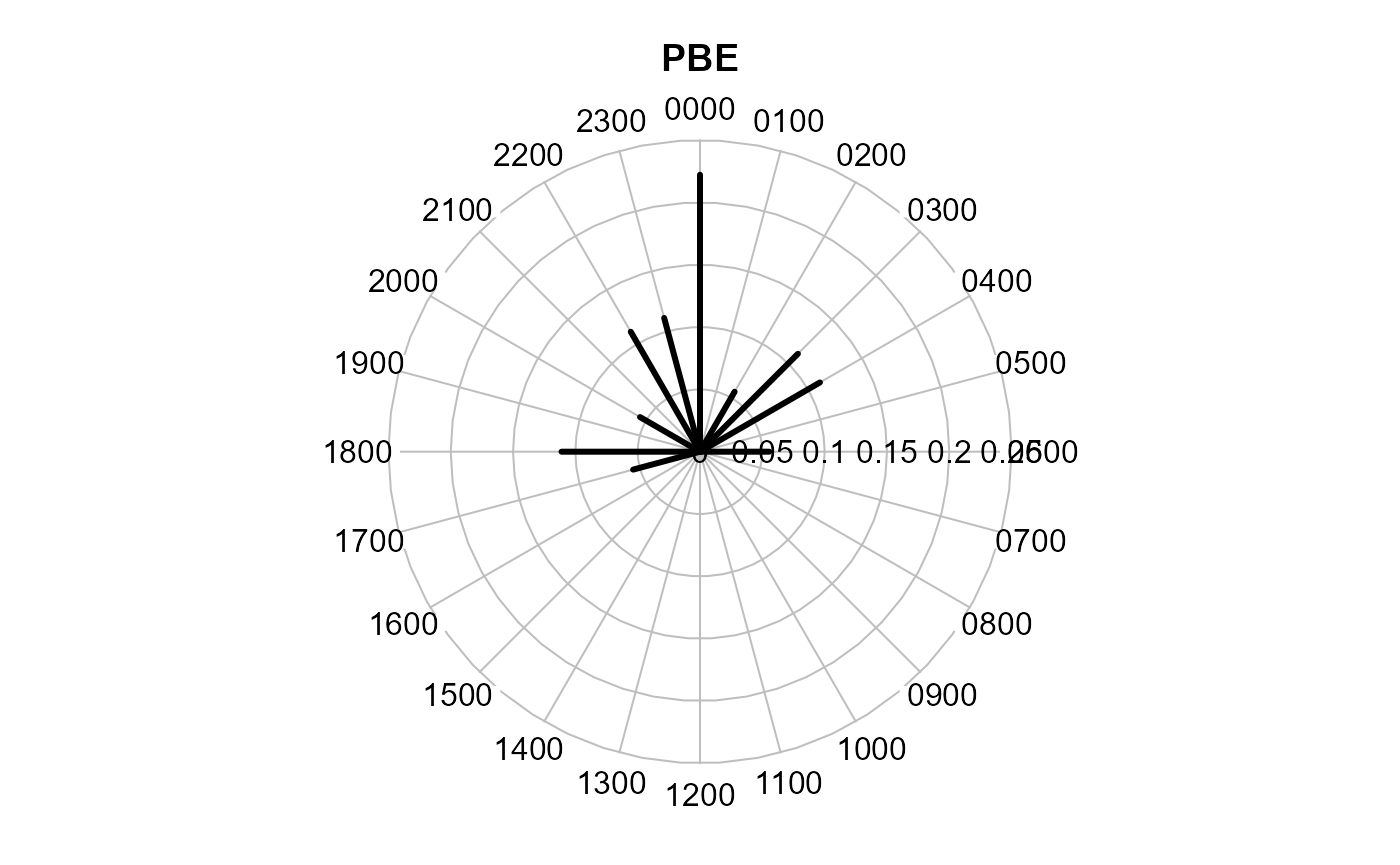
# we first pick a species for our activity trials
species4activity <- "PBE"    # = Prionailurus bengalensis, Leopard Cat
Kernel density estimation
activityDensity uses the function
densityPlot from the overlap package.
activityDensity(recordTable = recordTableSample,
                species     = species4activity)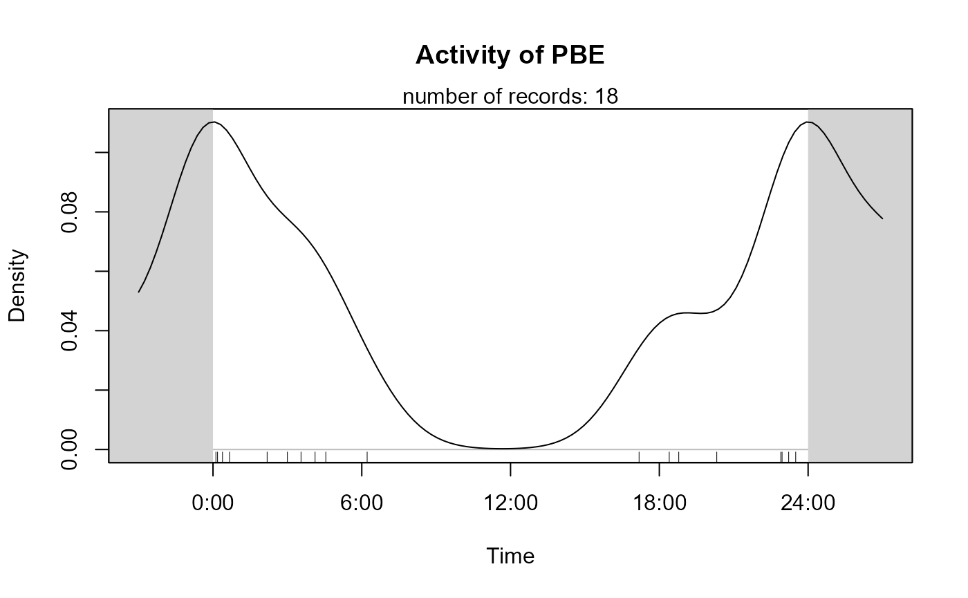
Histogram
This function creates a histogram with hourly intervals, i.e. histogram cells are 1 hour wide.
activityHistogram (recordTable = recordTableSample,
                   species     = species4activity)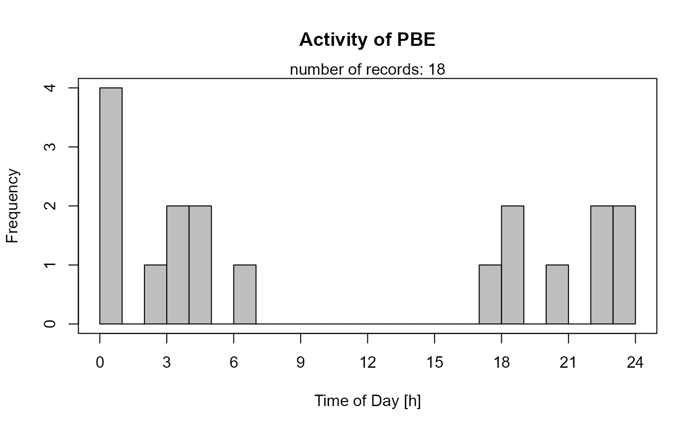
Radial plot
This function uses functions from the plotrix package to
create the clock face. Records are aggregated to the full hour (as in
activityHistogram).
activityRadial(recordTable  = recordTableSample,
               species      = species4activity,
               lwd          = 3       # adjust line with of the plot
)
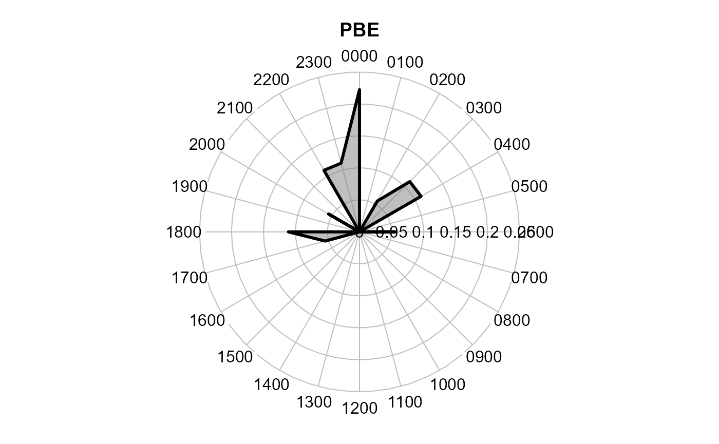
One can also make the function show a polygon instead of the radial
lines. rp.type is an argument to radial.plot
and defaults to "r" (radial). Setting it to
"p" gives a polygon. poly.col is optional and defines the
fill color of the polygon.
activityRadial(recordTable       = recordTableSample,
               species           = species4activity,
               allSpecies        = FALSE,
               speciesCol        = "Species",
               recordDateTimeCol = "DateTimeOriginal",
               plotR             = TRUE,
               writePNG          = FALSE,
               lwd               = 3,
               rp.type           = "p",     # plot type = polygon
               poly.col          = gray(0.5, alpha = 0.5)  # optional. remove for no fill
)
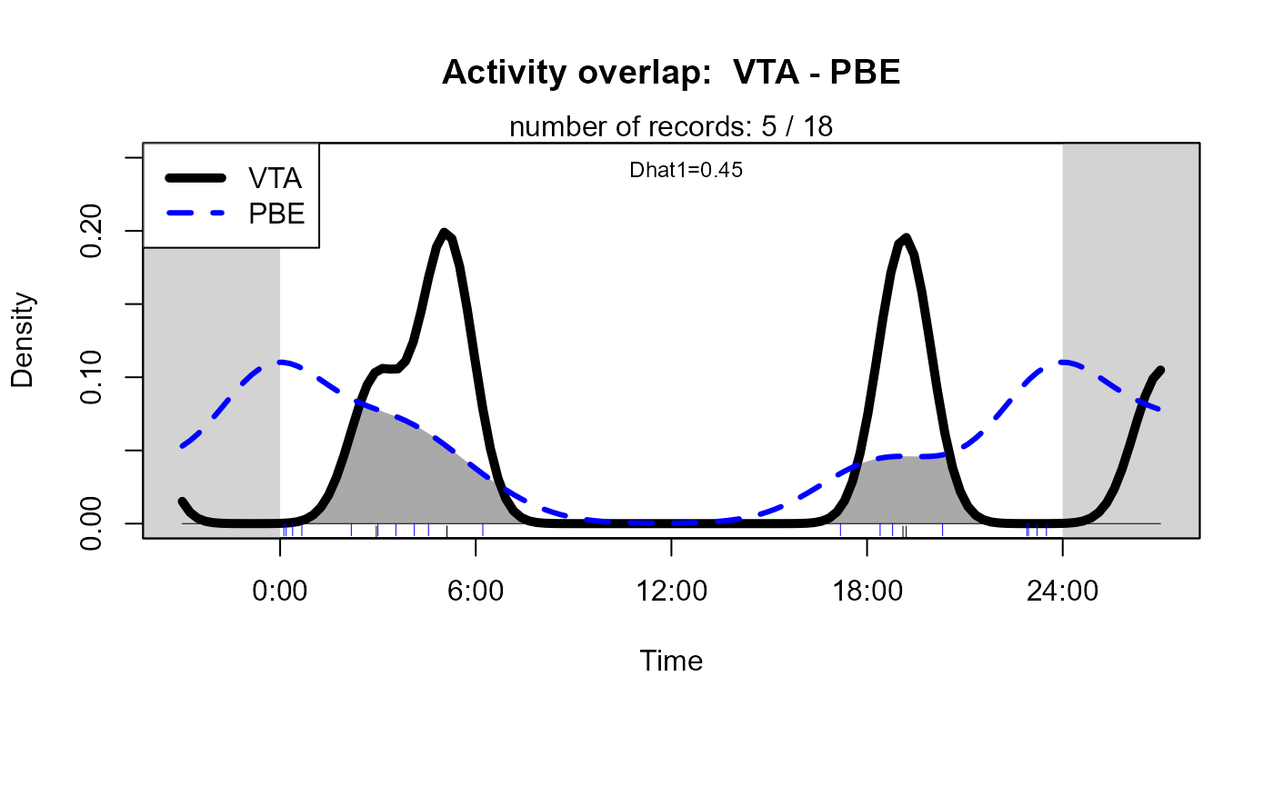
Two-species activity plots
Two-species activity overlaps can be plotted in addition to
single-species activity plots. It is the overlap between two
single-species kernel density estimations. The functions
overlapPlot and overlapEst from the
overlap package are used for that purpose. The overlap
coefficient shown in the plot is Dhat1 from overlapEst.
# define species of interest
speciesA_for_activity <- "VTA"    # = Viverra tangalunga, Malay Civet
speciesB_for_activity <- "PBE"    # = Prionailurus bengalensis, Leopard Cat

# create activity overlap plot
activityOverlap (recordTable = recordTableSample,
                 speciesA    = speciesA_for_activity,
                 speciesB    = speciesB_for_activity,
                 writePNG    = FALSE,
                 plotR       = TRUE,
                 add.rug     = TRUE
)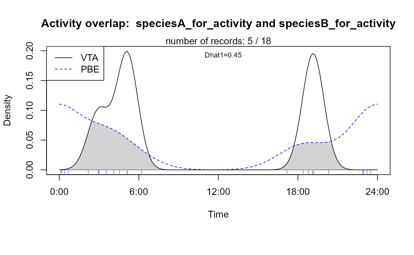
This plot an be customised by passing additional arguments to
overlapPlot:
activityOverlap (recordTable = recordTableSample,
                 speciesA    = speciesA_for_activity,
                 speciesB    = speciesB_for_activity,
                 writePNG    = FALSE,
                 plotR       = TRUE,
                 createDir   = FALSE,
                 pngMaxPix   = 1000,
                 linecol     = c("black", "blue"),
                 linewidth   = c(5,3),
                 linetype    = c(1, 2),
                 olapcol     = "darkgrey",
                 add.rug     = TRUE,
                 extend      = "lightgrey",
                 ylim        = c(0, 0.25),
                 main        = paste("Activity overlap: ", speciesA_for_activity, "-", speciesB_for_activity)
)
Survey summary report
surveyReport conveniently creates a summary report
containing:
- number of stations (total and operational)
- number of active trap days (total and by station)
- number of days with cameras set up (operational or not; total and by station)
- number of active trap days (taking into account multiple cameras accumulating effort independently at the same station)
- total trapping period
- camera trap and record date ranges
- number of species by station
- number of independent events by species
- number of stations at which species were recorded
- number of independent events by station and species
It requires a record table, the camera trap table, and (since version 2.1) a camera operation matrix.
The camera operation matrix is required to provide more precise and flexible calculation of the number of active trap days. So we first create the camera operation matrix, here taking into account periods in which the cameras malfunctioned (hasProblems = TRUE).
camop_problem <- cameraOperation(CTtable      = camtraps,
                                 stationCol   = "Station",
                                 setupCol     = "Setup_date",
                                 retrievalCol = "Retrieval_date",
                                 hasProblems  = TRUE,
                                 dateFormat   = "dmy")
reportTest <- surveyReport (recordTable          = recordTableSample,
                            CTtable              = camtraps,
                            camOp                = camop_problem,   # new argument since v2.1
                            speciesCol           = "Species",
                            stationCol           = "Station",
                            setupCol             = "Setup_date",
                            retrievalCol         = "Retrieval_date",
                            CTDateFormat         = "%d/%m/%Y",
                            recordDateTimeCol    = "DateTimeOriginal",
                            recordDateTimeFormat = "%Y-%m-%d %H:%M:%S" #,
                            #CTHasProblems        = TRUE    # deprecated in v2.1
                            )
##
## -------------------------------------------------------
## [1] "Total number of stations: 3"
##
## -------------------------------------------------------
## [1] "Number of operational stations: 3"
##
## -------------------------------------------------------
## [1] "Trap nights (number of active 24 hour cycles completed by independent cameras): 122.5"
##
## -------------------------------------------------------
## [1] "Calendar days with cameras set up (operational or not): 131"
##
## -------------------------------------------------------
## [1] "Calendar days with cameras set up and active: 125"
##
## -------------------------------------------------------
## [1] "Calendar days with cameras set up but inactive: 6"
##
## -------------------------------------------------------
## [1] "total trapping period: 2009-04-02 - 2009-05-17"Some basic information is shown in the console. The function output is a list with 5 elements.
str(reportTest)## List of 5
## $ survey_dates :'data.frame': 3 obs. of 10 variables:
## ..$ Station : chr [1:3] "StationA" "StationB" "StationC"
## ..$ setup : Date[1:3], format: "2009-04-02" "2009-04-03" ...
## ..$ retrieval : Date[1:3], format: "2009-05-14" "2009-05-16" ...
## ..$ image_first : Date[1:3], format: "2009-04-10" "2009-04-05" ...
## ..$ image_last : Date[1:3], format: "2009-05-07" "2009-05-14" ...
## ..$ n_cameras : int [1:3] 1 1 1
## ..$ n_calendar_days_total : num [1:3] 43 44 44
## ..$ n_calendar_days_active : num [1:3] 43 44 38
## ..$ n_calendar_days_inactive: num [1:3] 0 0 6
## ..$ n_trap_nights_active : num [1:3] 42 43 37.5
## $ species_by_station:'data.frame': 3 obs. of 2 variables:
## ..$ Station : chr [1:3] "StationA" "StationB" "StationC"
## ..$ n_species: int [1:3] 2 3 4
## $ events_by_species :'data.frame': 5 obs. of 3 variables:
## ..$ species : chr [1:5] "EGY" "MNE" "PBE" "TRA" ...
## ..$ n_events : chr [1:5] "6" "2" "18" "8" ...
## ..$ n_stations: chr [1:5] "1" "1" "3" "1" ...
## $ events_by_station :'data.frame': 9 obs. of 3 variables:
## ..$ Station : chr [1:9] "StationA" "StationA" "StationB" "StationB" ...
## ..$ Species : chr [1:9] "PBE" "VTA" "MNE" "PBE" ...
## ..$ n_events: int [1:9] 4 2 2 8 2 6 6 8 1
## $ events_by_station2:'data.frame': 15 obs. of 3 variables:
## ..$ Station : Factor w/ 3 levels "StationA","StationB",..: 1 1 1 1 1 2 2 2 2 2 ...
## ..$ Species : Factor w/ 5 levels "EGY","MNE","PBE",..: 1 2 3 4 5 1 2 3 4 5 ...
## ..$ n_events: num [1:15] 0 0 4 0 2 0 2 8 0 2 ...The list elements can be accessed individually like this:
reportTest[[1]] or like this:
reportTest$survey_dates.
Some of the arguments need further explanations.
If there was more than one camera per station cameraCol
specifies the columns containing camera IDs . Not setting it will cause
camtrapR to assume there was 1 camera per station, biasing the trap day
calculation. sinkpath can optionally be a directory in
which the function will save the output as a txt file.
# here's the output of surveyReport

reportTest[[1]]    # camera trap operation times and image date ranges
## Station setup retrieval image_first image_last n_cameras
## 1 StationA 2009-04-02 2009-05-14 2009-04-10 2009-05-07 1
## 2 StationB 2009-04-03 2009-05-16 2009-04-05 2009-05-14 1
## 3 StationC 2009-04-04 2009-05-17 2009-04-06 2009-05-12 1
## n_calendar_days_total n_calendar_days_active n_calendar_days_inactive
## 1 43 43 0
## 2 44 44 0
## 3 44 38 6
## n_trap_nights_active
## 1 42.0
## 2 43.0
## 3 37.5
reportTest[[2]] # number of species by station## Station n_species
## 1 StationA 2
## 2 StationB 3
## 3 StationC 4
reportTest[[3]] # number of events and number of stations by species## species n_events n_stations
## 1 EGY 6 1
## 2 MNE 2 1
## 3 PBE 18 3
## 4 TRA 8 1
## 5 VTA 5 3
reportTest[[4]] # number of species events by station## Station Species n_events
## 1 StationA PBE 4
## 2 StationA VTA 2
## 3 StationB MNE 2
## 4 StationB PBE 8
## 5 StationB VTA 2
## 6 StationC EGY 6
## 7 StationC PBE 6
## 8 StationC TRA 8
## 9 StationC VTA 1
# reportTest[[5]] is identical to reportTest[[4]] except for the fact that it contains unobserved species with n_events = 0